
Reconstructing the Wiring of a Nervous System
Instructors: Erik Jorgensen (Biology) and Tolga Tasdizen (Computer Science).
Assistants: Shigeki Watanabe (Biology) and Liz Jurrus (Computer Science).
The Class
In Spring Semester of 2010, the goal of Biological Microscopy was to use machine learning to reconstruct the wiring of a simple nervous system. The class was designed to bring together Biology majors and Computer Science majors to solve a problem requiring the expertise of these very different areas. Biologists learned how to acquire images of the nerve bundles using an electron microscope. Computer Science majors used machine-learning paradigms to recognize axon profiles, to convert these profiles into outlines and to automatically assemble cross-sections into reconstructed neurons.
The Problem
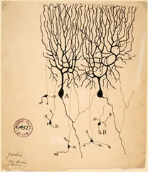
Figure 1: Illustration of a Purkinje cell
by Ramón y Cajal (1899).
Complex behaviors of an organism are governed by the nervous system. To fully understand how the neural circuit processes information it is necessary to know the connections between neurons in the circuit. Electron microscopy (EM) can be used to determine connectivity because it has a resolution that is high enough to identify direct connections between neurons: synapses and gap junctions. However, the reconstruction of a nervous system from serial electron micrographs may at first blush appear to be impossible. There are several problems that arise from the biology itself. First, neurons possess an extraordinarily complicated morphology. Such complexity can be recognized even in the illustrations from Santiago Ramón y Cajal at the turn of the century (Figure 1). Second, the wiring of the nervous system is the result of many stochastic developmental events. Nervous system wiring is in part a competitive process among cells that provides many solutions to a set of roughly defined rules. These rules guarantee a robustness to brain development although it may not produce the exact same solution in even genetically identical nervous systems. Thus, there is no standard reference brain anatomy. And once you have documented the connectivity pattern of a particular nervous system, how do you know it is correct?
A Simple Nervous System
In contrast to other organisms, the nematode Caenorhabditis elegans possesses an invariant nervous system. There are only 302 neurons, every individual possesses each of these neurons, and they occupy fixed positions in the animal. For this reason, the only nervous system ever fully reconstructed is that of this nematode (White et al., 1986). Thus, the ‘mind of the worm’ provides us with a touchstone to determine if our reconstructions are correct.
The Goal
Despite the simplicity of C. elegans, the mapping of this simple nervous system, comprised of only 6000 synapses, took over 10 years. In comparison, more complex organisms possess thousands of neurons and millions of synapses, thereby making the manual reconstruction nearly impossible. Thus, computer-assisted reconstruction will be essential to tackle more complex nervous systems.
The goal of this class then was to first collect serial electron micrographs of the ventral nerve cord from C. elegans and second, to assemble these micrographs into a reconstructed nervous system using machine-learning algorithms.
Sectioning
Adult nematodes were frozen rapidly under high pressure. These samples were held at -90°C so that ice molecules were exchanged for the solvent acetone and the fixative osmium tetroxide. The temperature was slowly raised. The fixative was removed and the worms embedded in plastic. The plastic blocks were then sectioned into 50 nm sections using a diamond knife on a microtome (Figure 2). Ribbons of sections were mounted on tiny copper slot grids.
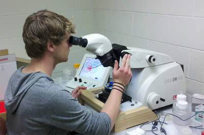
Figure 2: 50nm sections were cut using a diamond knife on a microtome.
Electron Microscopy
The grids with sections were mounted onto an armature and inserted into the electron microscope (Figure 3). The sections were exposed to an electron beam. Electron dense areas such as stained membranes cast a shadow and these images can be acquired on a CCD digital camera.
Figure 3: Cross-sections of the ventral nerve cord were acquired on a Hitachi 125keV electron microscope.
Machine Vision
Computational processing for the recognition of neurons is different from our visual processing. When we look at a set of images, we immediately recognize each axon profile by the thickness and intensity of the membrane, the circular shapes of the processes – even if incomplete, and ignore visual noise in the image like tears or folds in the section. We are also not confused by cross-sections of mitochondria which are nicely circular but somewhat darker in staining intensity. We can also follow particular processes through multiple sections based on the shape location of the neurons relative to other features in the images. However, a computer must look at each pixel in an image and assign it to a membrane, and reconstruct the path of that membrane. Then based on the position of the cell membrane in the image, a computer must find the same neuron in the next image.
The automated reconstruction processes thus requires five steps: image alignment, membrane detection, tracing axon profiles in a single section (2D segmentation), linking of axon profiles between sections (3D segmentation), and volume rendering.
Alignment
The students acquired over 1500 serial images from the ventral nerve cord of C. elegans. These images then had to be aligned. Because the imaging field was user-defined, the ventral nerve cord in every section was not necessarily in the center of the picture with the same orientation (Figure 4, top). Therefore, the images had to be aligned. This process was automated by using ir-tools], developed by the Scientific Computing and Imaging Institute (SCI) at the University of Utah (Figure 4 bottom). The aligned dataset was used for the development of the computational membrane detection algorithm.
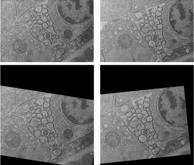
Figure 4: Two consecutive sections of the ventral nerve cord. (Top) raw images. Notice that the image on right is slightly shifted and rotated compared to the image on left. (Bottom) after automated alignment.
Membrane Detection
A computer must look at the grayscale value of each pixel in an image and determine if the particular pixel is a part of a membrane based on local context (Figure 5).

Figure 5: The contexts recognized by a computer. A computer must distinguish the neuronal membrane at this level.
Unevenness in illumination intensity was removed globally. The contrast was then increased to enhance local features, and the images down-sampled to increase processing speed. Membranes were detected due to their anisotropic nature, that is, they extend in a single dimension. Membrane continuity was improved by enhancing pixels extending from a trajectory. Sample datasets were analyzed by the computer, and with multiple rounds of training, the computer was able to recognize axon membranes (Figure 6).
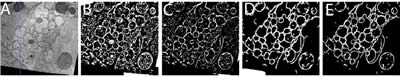
Figure 6: Machine detection. (A) Raw data (B) Thresholding and anisotropic smoothing (C) Membrane detection using Hessian eigenvalues (D) Serial training with filter banks (E) Serial training with stencils.
2D Segmentation
Axons are identified using a flood fill protocol. In short, pixels are colored starting at low intensities and include neighboring pixels as pixel intensities increase. Dark membranes represent walls that confine flooding to single axon profiles. Flood levels are determined by the operator to maximize the accuracy of the segmentation compared to the training sets (Figure 7).
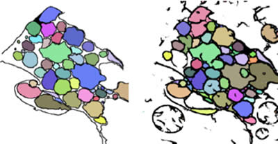
Figure 7: A comparison between hand-segmented axons (left) and machine-segmented axons following a flood fill (right).
3D Segmentation
The profiles identified in serial sections must now be connected together to form axons. When we look at serial sections, we can easily follow particular processes through the images based on the shape of neuron and the location of the neurons relative to other features in the images. However, a computer must compare the axon profiles, and even though they may have changed position and shape, the computer must select the most probable profile among the axons in the next image. If a particular section was difficult to segment in two dimensions, then there may be fewer or greater axon profiles in the next image.
Profiles in one section are compared to profiles in an adjacent section. First, two profiles must match each others’ shapes when stacked on top of one another. Second, profiles are linked using a shortest-path algorithm. Jumps to distant profiles are punished. Then axon trajectories are identified in the entire volume (Figure 8, left).
Visualization
The computer now has determined the three dimensional structure of the axons. Now the reconstruction must be portrayed to the viewer. Axon membranes serve as nodes that connect edges to the next section. In our reconstruction, 24 axons in the ventral nerve cord were reconstructed and visualized from the dataset acquired during the class (Figure 8, right).
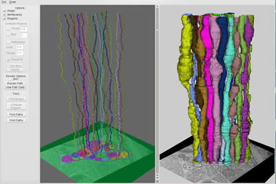
Figure 8: NeRV - Neuron Reconstruction Viewer. 24 axons in the ventral nerve cord were reconstructed in a semi-automated fashion (left) and three dimensional volumes rendered (right).