
Super-Resolution Microscopy Tutorial
Overview
Super-resolution microscopy is a collective name for a number of techniques that achieve resolution below the conventional resolution limit, defined as the minimum distance that two point-source objects have to be in order to distinguish the two sources from each other. There are two closely related values for the diffraction limit, the Abbe and Rayleigh criterions. The difference between the two is based on the definition that both Abbe and Rayleigh used in their derivation for what is meant by two objects being resolvable from each other. In practical applications, this difference is small. The Abbe criterion is defined as:
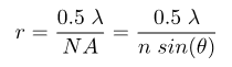
while the Rayleigh criterion defines the resolution mathematically as:
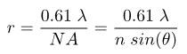
where r is the distance the two objects are from each other, λ is the wavelength of light, n is the index of refraction of the medium between the objective and the sample, and NA is the numerical aperture of the objective lens that collects light. Specifically, the numerical aperture is the collection angle of light that enters the objective, as given by the angle θ in the figure below. The difference in the two is the value of the coefficient, which is a result of the difference in how Abbe and Rayleigh defined what it means for two distinct objects to be resolved from each other (more on this later). For a point source radiating light at a wavelength of 510 nm and a microscope objective with a numerical aperture (NA) value of 1.4, the value of r from the Rayleigh equation will be 222 nm. The rest of this tutorial will assume the Rayleigh criterion as the standard definition of the resolution limit.
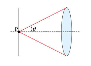
Figure 1: Graphical diagram of the definition of numerical aperture.
The diffraction limit arises due to the wave nature of light and its interaction with the optical systems it passes through, namely the diffraction, or scattering, of the incoming light, that occurs at the entrance to the microscope objective. This phenomenon results in a loss of information with regards to the true location of a point source that is emitting light, say for instance a molecule of green fluorescent protein (GFP). For example, a single GFP fluorescent protein, emitting light at a wavelength of 510 nm, will give rise to an intensity distribution on a camera that is known as the Airy pattern, a diffuse, delocalized and symmetric pattern of light with a radius of 222 nm, as defined in the Rayleigh criterion above. This pattern is shown below in Figure 2.
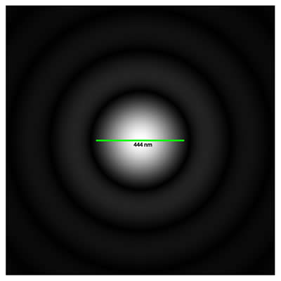
Figure 2: Intensity profile of a single fluorophore emitting light onto a CCD camera; this is known as the Airy pattern. The fluorophore is at the center of the image, and can be considered a point source. For GFP emitting at a peak of 510 nm, and an objective numerical aperture of 1.4, the width of this intensity profile will be 444 nm. This profile is a result of the wave nature of light as the photons from the fluorescent protein diffract (scatter) off of the aperture of the objective and interfere with each other. Thus, a point source (the fluorescent protein) is no longer viewed as a point source, but rather as a diffuse, delocalized intensity pattern.
The profile of this two dimensional pattern is shown below in Figure 3.
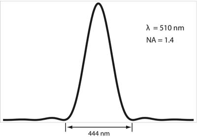
Figure 3: Profile along the green line shown above in Figure 2.
This disparity in size between the physical dimensions of the GFP molecule (roughly 2-4 nm) to the size of the diffraction pattern (roughly 450 nm across) underlies the resolution limit in conventional optical microscopy. If we were to compare the sizes of the two next to each other, we would observe something like the following figure:
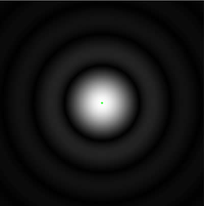
Figure 4: Size of GFP in relation to the Airy pattern that its emitted light produces on a CCD camera. The GFP protein is the small green dot in the center of the image. In practical terms, the image on a camera will be both pixelated, and have a larger background in the image, making the ring pattern difficult to observe experimentally.
As one can see, the intensity pattern of light onto the camera is much larger than the physical size of the protein, and if we had two such proteins, or 10 such proteins, within this single Airy profile, we would not be able to resolve the individual proteins from each other. This is the idea of the resolution limit: the physical distance in space that two such point sources would have to lie in order to distinguish their individual light intensity pattern, or their point spread function (PSF), from each other. There are a few criterions for such resolution limits; the Rayleigh and Abbe criterions, as described above, as well as the Sparrow criterion. Examples of the three different types are given below by the following figure. The Sparrow is used more often in astronomy, while the Rayleigh and Abbe criterion are more conventional in microscopy.

Figure 5: Various conventional resolution limits and their definitions. In the Rayleigh convention, the first minimum of one Airy profile overlaps the maximum of the second Airy profile, with the sum of the two profiles showing a distinct dip. In the Sparrow criterion, the sum of the two Airy patterns produces a flat intensity profile; in the Abbe limit, a small dip is still discernible between the two maxima.
Two main types of super-resolution microscopy have emerged in the past few years that are able to achieve resolution limits beyond the values described above. The first method developed is known as stimulated emission depletion microscopy, or STED microscopy, and was invented and pioneered by Dr. Stefan Hell of the Max Planck Institute for Biophysical Chemistry in Göttingen, Germany. For information relating to this technique, which relies on point spread function engineering to break the conventional diffraction limit, please see Dr. Hell's group page.
The other variant of super-resolution microscopy is known as PALM (photo-activated localization microscopy) and was developed by Eric Betzig and Harald Hess of Howard Hughes Medical Institutes' Janelia Farm Research Campus and independently by Sam Hess (no relation) of the University of Maine. This technique takes advantage of the new generation of photo-activatible and photo-switchable proteins that have been developed in the past few years. Under irradiation by UV light, these proteins undergo a chemical conversion and switch from one particular state to another. In the case of photo-activatible proteins, they undergo a conversion from a dark 'off' state to a bright 'on' state. For photo-switchable fluorophores, they will switch from one color to another color; this process may or may not be reversible, depending on the fluorophore in question. In the examples below, the fluorophore EOS will undergo a conversion from a green state to a red state.
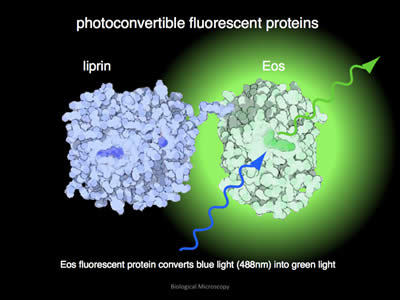
Figure 6: In its unconverted format, EOS will glow green when illuminated with blue light. In this example, the fluorophore EOS has been attached to the protein liprin.
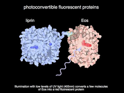
Figure 7: Under illumination with UV light, the EOS fluorophore converts from its green state to a red state. The fluorophore undergoes a chemical rearrangement due to irradiation by UV light, and as such, its fluorescent spectrum shifts from green to red.
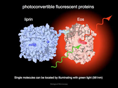
Figure 8: After conversion, when illuminated with green light, EOS will emit red light.
If the level of UV light is kept at a very low level, the number of fluorophores converted from an 'off' to an 'on' state is low across the volume of the sample being imaged, and most importantly, the probability of two individual fluorophores being activated within a region smaller than the diffraction limit from each other is very small, and thus each diffraction-limited spot imaged on the camera is due to the emission of one fluorophore. Since the intensity pattern of a point source is exactly known analytically, the experimentally measured point spread function can be computationally localized via fitting algorithms that fit the measured point spread function to a theoretical point spread function. While the STED technique knows a priori where the emitted fluorescence is emitted from due to the nature of the scanning method used in the image technique, the PALM methodology relies on randomly activated fluorophores being localized, and an image is built up by successively imaging a large number of frames and compiling a composite picture. This technique is outlined in the figures below.
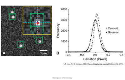
Figure 9: In the left image, the raw readout from a CCD camera shows the light pattern from four distinct fluorescent molecules that have undergone photo-activation. These fluorescent patterns obey well-known laws of physics, and as such, can be modeled mathematically. Thus, the raw data can be fit to a mathematical formula, and the peak of this photon distribution, as shown on the right, can be extracted, giving the location of the individual fluorophore. Image taken from: S.T.Hess, T.P.K. Girirajan, M.D. Mason, Biophysical Journal 91(11), 4258-4272 (2006).
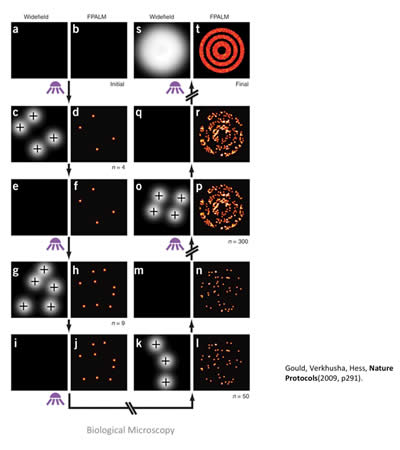
Figure 10: In this cartoon, the imaging sequence of the PALM method is outlined. Starting from the left two columns and following the arrows, a small subset of fluorophores is activated (diffuse white circles) and then localized via a computer-fitting algorithm (small red dots). After each cycle, the fluorophores are photo-bleached, or break down, and no longer emit fluorescence, so no two fluorophores are imaged twice. After thousands of cycles, a composite image is built up (top right, bulls-eye), showing much more detail and structure than the large diffuse blob that would be seen if all fluorophores were activated and fluorescent at one time. Cartoon taken from: T. J. Gould, V. V. Verkhusha, S.T. Hess, Nature Protocols 4, 291-308 (2009).
With such techniques, one can create images such as the following:
Conventional vs. PALM Imaging
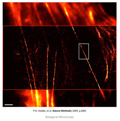
Figure 11: TIRFM (top and bottom) and PALM (middle) overlay image of stress fibers (actin bundles) labeled with EOS in a live HeLa cell. The top and bottom show conventional diffraction limit imaging, while the middle shows post-processing and the increase in resolution. Scale bar is 2 μm. Taken from: P. N. Hedde, et. al. Nature Methods 6, 689-690 (2009).
Up to this point, the methods for creating PALM microscopes have employed widefield microscopy, wherein the entire sample is bathed in light simultaneously. Conventional confocal and STED microscopy employ scanning techniques, wherein only a small region is illuminated at a given time as the focused beam is moved across the sample. One of the downsides to the PALM technique is that fluorescent proteins are not robustly photo-stable fluorophores, and they readily break down under harsh illumination conditions. By combining a scanning system with the PALM technique, we plan to build a microscope that increases the photon-yield from individual proteins, thereby increasing the resolving power of the PALM technique.